Pandas Basics 1
pandas Series와 DataFrame 생성, 조회, 정렬, 함수 적용
pandas 데이터 구조
- Series : 1D 동질의 데이터 타입을 갖는 배열(array)
- DataFrame : 2D 테이블 구조. 각 컬럼은 서로 다른 데이터타입을 가질 수 있음.
- Panel : 3D 테이블 구조.
import pandas as pd
import numpy as np
객체 생성
1. Series
s = pd.Series([1,3,5,np.nan,6,8])
s
0    1.0
1    3.0
2    5.0
3    NaN
4    6.0
5    8.0
dtype: float64
s.index
RangeIndex(start=0, stop=6, step=1)
s2 = pd.Series([4, 7, -5, 3], index=['d', 'b', 'a', 'c'])   # 인덱스 지정
s2
d    4
b    7
a   -5
c    3
dtype: int64
s2['a'] # 인덱스로 값 선택
-5
# Dictionary to Series
europe = {'spain': 46.77, 'france': 66.03, 'germany': 80.62, 'norway': 5.084}
s3 = pd.Series(europe)
s3
france     66.030
germany    80.620
norway      5.084
spain      46.770
dtype: float64
2. DataFrame
# row, column 데이터 지정하여 생성
dates = pd.date_range('20161001', periods=7)
dates
DatetimeIndex(['2016-10-01', '2016-10-02', '2016-10-03', '2016-10-04',
               '2016-10-05', '2016-10-06', '2016-10-07'],
              dtype='datetime64[ns]', freq='D')
# 랜덤으로 소수점 2자리 수 생성하여 각 컬럼의 값으로 사용
df = pd.DataFrame(np.random.rand(7,4).round(2), index=dates, columns=list('ABCD'))
df
| A | B | C | D | |
|---|---|---|---|---|
| 2016-10-01 | 0.87 | 0.06 | 0.03 | 0.56 |
| 2016-10-02 | 0.71 | 0.37 | 0.26 | 0.06 |
| 2016-10-03 | 0.98 | 0.53 | 0.88 | 0.30 |
| 2016-10-04 | 0.10 | 0.16 | 0.02 | 0.90 |
| 2016-10-05 | 0.20 | 0.64 | 0.36 | 0.54 |
| 2016-10-06 | 0.49 | 0.50 | 0.66 | 0.21 |
| 2016-10-07 | 0.54 | 0.05 | 0.33 | 0.63 |
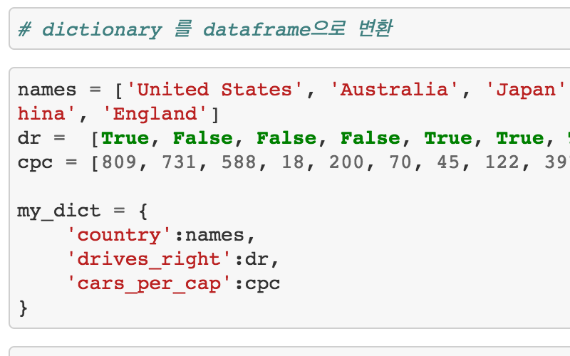
# dictionary 를 dataframe으로 변환
names = ['United States', 'Australia', 'Japan', 'India', 'Russia', 'Morocco', 'Egypt', 'Korea', 'China', 'England']
dr =  [True, False, False, False, True, True, True, True, True, True]
cpc = [809, 731, 588, 18, 200, 70, 45, 122, 397, 255]

my_dict = {
    'country':names,
    'drives_right':dr,
    'cars_per_cap':cpc
}
cars = pd.DataFrame(my_dict)
cars
| cars_per_cap | country | drives_right | |
|---|---|---|---|
| 0 | 809 | United States | True |
| 1 | 731 | Australia | False |
| 2 | 588 | Japan | False |
| 3 | 18 | India | False |
| 4 | 200 | Russia | True |
| 5 | 70 | Morocco | True |
| 6 | 45 | Egypt | True |
| 7 | 122 | Korea | True |
| 8 | 397 | China | True |
| 9 | 255 | England | True |
# dataframe 구조 보기
cars.dtypes
cars_per_cap     int64
country         object
drives_right      bool
dtype: object
cars.shape
(10, 3)
데이터 조회
cars.head()
| cars_per_cap | country | drives_right | |
|---|---|---|---|
| 0 | 809 | United States | True |
| 1 | 731 | Australia | False |
| 2 | 588 | Japan | False |
| 3 | 18 | India | False |
| 4 | 200 | Russia | True |
cars.tail(3)
| cars_per_cap | country | drives_right | |
|---|---|---|---|
| 7 | 122 | Korea | True |
| 8 | 397 | China | True |
| 9 | 255 | England | True |
cars.index # 각 행의 인덱스
RangeIndex(start=0, stop=10, step=1)
cars.columns # 컬럼명
Index(['cars_per_cap', 'country', 'drives_right'], dtype='object')
cars.values # 전체 데이터 조회
array([[809, 'United States', True],
       [731, 'Australia', False],
       [588, 'Japan', False],
       [18, 'India', False],
       [200, 'Russia', True],
       [70, 'Morocco', True],
       [45, 'Egypt', True],
       [122, 'Korea', True],
       [397, 'China', True],
       [255, 'England', True]], dtype=object)
cars.T # transposing data
| 0 | 1 | 2 | 3 | 4 | 5 | 6 | 7 | 8 | 9 | |
|---|---|---|---|---|---|---|---|---|---|---|
| cars_per_cap | 809 | 731 | 588 | 18 | 200 | 70 | 45 | 122 | 397 | 255 |
| country | United States | Australia | Japan | India | Russia | Morocco | Egypt | Korea | China | England |
| drives_right | True | False | False | False | True | True | True | True | True | True |
cars.describe() # 요약된 통계 정보
| cars_per_cap | |
|---|---|
| count | 10.000000 |
| mean | 323.500000 |
| std | 293.035929 |
| min | 18.000000 |
| 25% | 83.000000 |
| 50% | 227.500000 |
| 75% | 540.250000 |
| max | 809.000000 |
df.describe()
| A | B | C | D | |
|---|---|---|---|---|
| count | 7.000000 | 7.000000 | 7.000000 | 7.000000 |
| mean | 0.555714 | 0.330000 | 0.362857 | 0.457143 |
| std | 0.326948 | 0.240416 | 0.315104 | 0.284881 |
| min | 0.100000 | 0.050000 | 0.020000 | 0.060000 |
| 25% | 0.345000 | 0.110000 | 0.145000 | 0.255000 |
| 50% | 0.540000 | 0.370000 | 0.330000 | 0.540000 |
| 75% | 0.790000 | 0.515000 | 0.510000 | 0.595000 |
| max | 0.980000 | 0.640000 | 0.880000 | 0.900000 |
df.mean(axis='columns') # 전체 컬럼의 평균
2016-10-01    0.3800
2016-10-02    0.3500
2016-10-03    0.6725
2016-10-04    0.2950
2016-10-05    0.4350
2016-10-06    0.4650
2016-10-07    0.3875
Freq: D, dtype: float64
df.mean(axis='rows') # 각 컬럼별 행의 평균
A    0.555714
B    0.330000
C    0.362857
D    0.457143
dtype: float64
Reindex
obj = pd.Series([4.5, 7.2, -5.3, 3.6], index=['d', 'b', 'a', 'c'])
obj
d    4.5
b    7.2
a   -5.3
c    3.6
dtype: float64
obj.reindex(['a', 'b', 'c', 'd', 'e'])
a   -5.3
b    7.2
c    3.6
d    4.5
e    NaN
dtype: float64
obj.reindex(['a', 'b', 'c', 'd', 'e'], fill_value=0)
a   -5.3
b    7.2
c    3.6
d    4.5
e    0.0
dtype: float64
함수 적용
dates = pd.date_range('20161011', periods=7)
df = pd.DataFrame(np.random.rand(7,4).round(4), index=[dates], columns=list('DABC'))
df
| D | A | B | C | |
|---|---|---|---|---|
| 2016-10-11 | 0.9553 | 0.3991 | 0.1396 | 0.6029 |
| 2016-10-12 | 0.6353 | 0.3549 | 0.2553 | 0.5542 |
| 2016-10-13 | 0.2645 | 0.9218 | 0.8819 | 0.8357 |
| 2016-10-14 | 0.7968 | 0.2667 | 0.4447 | 0.6609 |
| 2016-10-15 | 0.7353 | 0.1914 | 0.5258 | 0.5743 |
| 2016-10-16 | 0.7666 | 0.3549 | 0.5251 | 0.0739 |
| 2016-10-17 | 0.3224 | 0.2378 | 0.6657 | 0.3437 |
f = lambda x: x.max() - x.min()
df.apply(f)
D    0.6908
A    0.7304
B    0.7423
C    0.7618
dtype: float64
df.apply(f, axis=1)
2016-10-11    0.8157
2016-10-12    0.3800
2016-10-13    0.6573
2016-10-14    0.5301
2016-10-15    0.5439
2016-10-16    0.6927
2016-10-17    0.4279
Freq: D, dtype: float64
def f2(x):
    return pd.Series([x.min(), x.max()], index=['min', 'max'])
df.apply(f2)
| D | A | B | C | |
|---|---|---|---|---|
| min | 0.2645 | 0.1914 | 0.1396 | 0.0739 |
| max | 0.9553 | 0.9218 | 0.8819 | 0.8357 |
# dataframe의 실수값을 문자열로 일괄 변환
f_form = lambda x: '%.2f' % x
df.applymap(f_form)
| D | A | B | C | |
|---|---|---|---|---|
| 2016-10-11 | 0.96 | 0.40 | 0.14 | 0.60 |
| 2016-10-12 | 0.64 | 0.35 | 0.26 | 0.55 |
| 2016-10-13 | 0.26 | 0.92 | 0.88 | 0.84 |
| 2016-10-14 | 0.80 | 0.27 | 0.44 | 0.66 |
| 2016-10-15 | 0.74 | 0.19 | 0.53 | 0.57 |
| 2016-10-16 | 0.77 | 0.35 | 0.53 | 0.07 |
| 2016-10-17 | 0.32 | 0.24 | 0.67 | 0.34 |
정렬
# sort_index
df.sort_index(axis=1)
| A | B | C | D | |
|---|---|---|---|---|
| 2016-10-11 | 0.3991 | 0.1396 | 0.6029 | 0.9553 |
| 2016-10-12 | 0.3549 | 0.2553 | 0.5542 | 0.6353 |
| 2016-10-13 | 0.9218 | 0.8819 | 0.8357 | 0.2645 |
| 2016-10-14 | 0.2667 | 0.4447 | 0.6609 | 0.7968 |
| 2016-10-15 | 0.1914 | 0.5258 | 0.5743 | 0.7353 |
| 2016-10-16 | 0.3549 | 0.5251 | 0.0739 | 0.7666 |
| 2016-10-17 | 0.2378 | 0.6657 | 0.3437 | 0.3224 |
df.sort_index(axis=1, ascending=False) # 컬럼 순서 뒤집기
| D | C | B | A | |
|---|---|---|---|---|
| 2016-10-11 | 0.9553 | 0.6029 | 0.1396 | 0.3991 |
| 2016-10-12 | 0.6353 | 0.5542 | 0.2553 | 0.3549 |
| 2016-10-13 | 0.2645 | 0.8357 | 0.8819 | 0.9218 |
| 2016-10-14 | 0.7968 | 0.6609 | 0.4447 | 0.2667 |
| 2016-10-15 | 0.7353 | 0.5743 | 0.5258 | 0.1914 |
| 2016-10-16 | 0.7666 | 0.0739 | 0.5251 | 0.3549 |
| 2016-10-17 | 0.3224 | 0.3437 | 0.6657 | 0.2378 |
# sort_values : 특정 컬럼의 값을 기준으로 정렬
df.sort_values(by='C')
| D | A | B | C | |
|---|---|---|---|---|
| 2016-10-16 | 0.7666 | 0.3549 | 0.5251 | 0.0739 |
| 2016-10-17 | 0.3224 | 0.2378 | 0.6657 | 0.3437 |
| 2016-10-12 | 0.6353 | 0.3549 | 0.2553 | 0.5542 |
| 2016-10-15 | 0.7353 | 0.1914 | 0.5258 | 0.5743 |
| 2016-10-11 | 0.9553 | 0.3991 | 0.1396 | 0.6029 |
| 2016-10-14 | 0.7968 | 0.2667 | 0.4447 | 0.6609 |
| 2016-10-13 | 0.2645 | 0.9218 | 0.8819 | 0.8357 |
cars.sort_values(by='country')
| cars_per_cap | country | drives_right | |
|---|---|---|---|
| 1 | 731 | Australia | False |
| 8 | 397 | China | True |
| 6 | 45 | Egypt | True |
| 9 | 255 | England | True |
| 3 | 18 | India | False |
| 2 | 588 | Japan | False |
| 7 | 122 | Korea | True |
| 5 | 70 | Morocco | True |
| 4 | 200 | Russia | True |
| 0 | 809 | United States | True |
# rank
df.rank(method='first') # 값이 같은 경우 위치에 따라 순위 부여. (etc : average, min, max)
| D | A | B | C | |
|---|---|---|---|---|
| 2016-10-11 | 7.0 | 6.0 | 1.0 | 5.0 |
| 2016-10-12 | 3.0 | 4.0 | 2.0 | 3.0 |
| 2016-10-13 | 1.0 | 7.0 | 7.0 | 7.0 |
| 2016-10-14 | 6.0 | 3.0 | 3.0 | 6.0 |
| 2016-10-15 | 4.0 | 1.0 | 5.0 | 4.0 |
| 2016-10-16 | 5.0 | 5.0 | 4.0 | 1.0 |
| 2016-10-17 | 2.0 | 2.0 | 6.0 | 2.0 |
df.rank(axis=1)
| D | A | B | C | |
|---|---|---|---|---|
| 2016-10-11 | 4.0 | 2.0 | 1.0 | 3.0 |
| 2016-10-12 | 4.0 | 2.0 | 1.0 | 3.0 |
| 2016-10-13 | 1.0 | 4.0 | 3.0 | 2.0 |
| 2016-10-14 | 4.0 | 1.0 | 2.0 | 3.0 |
| 2016-10-15 | 4.0 | 1.0 | 2.0 | 3.0 |
| 2016-10-16 | 4.0 | 2.0 | 3.0 | 1.0 |
| 2016-10-17 | 2.0 | 1.0 | 4.0 | 3.0 |