Pandas Plotting 2
line chart, box plot, scatter plot, histogram, Rolling means (moving averages)
import pandas as pd
import numpy as np
%matplotlib inline
import matplotlib.pyplot as plt
# setting plot defatult size
%pylab inline
pylab.rcParams['figure.figsize'] = (12, 6)
Populating the interactive namespace from numpy and matplotlib
df = pd.read_csv('data/ind_pop_data.csv')
df.head()
| CountryName | CountryCode | Year | TotalPop | UrbanPopRatio | |
|---|---|---|---|---|---|
| 0 | Afghanistan | AFG | 1960 | 8990000.0 | 8.22 |
| 1 | Afghanistan | AFG | 1961 | 9160000.0 | 8.51 |
| 2 | Afghanistan | AFG | 1962 | 9340000.0 | 8.81 |
| 3 | Afghanistan | AFG | 1963 | 9530000.0 | 9.11 |
| 4 | Afghanistan | AFG | 1964 | 9730000.0 | 9.43 |
df.values
array([['Afghanistan', 'AFG', 1960, 8990000.0, 8.22],
       ['Afghanistan', 'AFG', 1961, 9160000.0, 8.51],
       ['Afghanistan', 'AFG', 1962, 9340000.0, 8.81],
       ...,
       ['Zimbabwe', 'ZWE', 2013, 14900000.0, 32.7],
       ['Zimbabwe', 'ZWE', 2014, 15200000.0, 32.5],
       ['Zimbabwe', 'ZWE', 2015, 15600000.0, 32.4]], dtype=object)
df.index
RangeIndex(start=0, stop=14612, step=1)
create dataframe from dictionary
#1. by zip lists
list_keys = ['country', 'population']
list_values = [['targaryen', 'stark'], [579, 973]]
zipped = list(zip(list_keys,list_values))
data = dict(zipped)
df_zip = pd.DataFrame(data)
df_zip
| country | population | |
|---|---|---|
| 0 | targaryen | 579 |
| 1 | stark | 973 |
df_zip.columns = ['kingdom', 'army'];   # change column labels
df_zip
| kingdom | army | |
|---|---|---|
| 0 | targaryen | 579 |
| 1 | stark | 973 |
# 2. by broadcasting
data = {'kingdom':list_values[0], 'babies':list_values[1]}
df_dict = pd.DataFrame(data)
df_dict
| babies | kingdom | |
|---|---|---|
| 0 | 579 | targaryen |
| 1 | 973 | stark |
Importing & Exporting
데이터가 깔끔하지 않은 파일에서 데이터 가져오기
# df1 = pd.read_csv(file_messy, header=0, names=new_col_names)
# df2 = pd.read_csv(file_messy, delimiter=' ', header=3, comment='#')
데이터 저장하기
# df2.to_csv(file_clean, index=False)              # Save the DataFrame to a CSV file without the index
# df2.to_excel('file_clean.xlsx', index=False)   # Save the DataFrame to an excel file without the index
Ploting with pandas
df_pop = pd.read_csv('data/ind_pop_data.csv')
df_pop.head()
| CountryName | CountryCode | Year | TotalPop | UrbanPopRatio | |
|---|---|---|---|---|---|
| 0 | Afghanistan | AFG | 1960 | 8990000.0 | 8.22 |
| 1 | Afghanistan | AFG | 1961 | 9160000.0 | 8.51 |
| 2 | Afghanistan | AFG | 1962 | 9340000.0 | 8.81 |
| 3 | Afghanistan | AFG | 1963 | 9530000.0 | 9.11 |
| 4 | Afghanistan | AFG | 1964 | 9730000.0 | 9.43 |
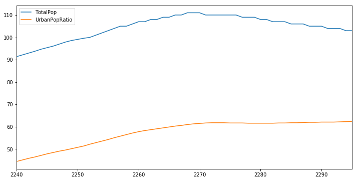
# example 1
df_c = df_pop[df_pop['CountryCode'] == 'CEB'].loc[:,['TotalPop','UrbanPopRatio']]
df_c.TotalPop = df_c.TotalPop / 1000000
df_c.head()
| TotalPop | UrbanPopRatio | |
|---|---|---|
| 2240 | 91.4 | 44.5 |
| 2241 | 92.2 | 45.2 |
| 2242 | 93.0 | 45.9 |
| 2243 | 93.8 | 46.5 |
| 2244 | 94.7 | 47.2 |
df_c.plot()
<matplotlib.axes._subplots.AxesSubplot at 0x10d612198>
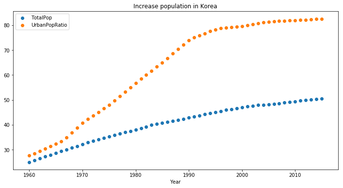
# example 2
df_k = df_pop[df_pop['CountryCode'] == 'KOR'].loc[:,['Year','TotalPop','UrbanPopRatio']]
df_k.TotalPop = df_k.TotalPop / 1000000
df_k.head()
| Year | TotalPop | UrbanPopRatio | |
|---|---|---|---|
| 6884 | 1960 | 25.0 | 27.7 |
| 6885 | 1961 | 25.8 | 28.5 |
| 6886 | 1962 | 26.5 | 29.5 |
| 6887 | 1963 | 27.3 | 30.4 |
| 6888 | 1964 | 28.0 | 31.4 |
plt.scatter(df_k['Year'], df_k['TotalPop'])
plt.scatter(df_k['Year'], df_k['UrbanPopRatio'])
plt.legend()
plt.title('Increase population in Korea')
plt.xlabel('Year')
<matplotlib.text.Text at 0x111580320>
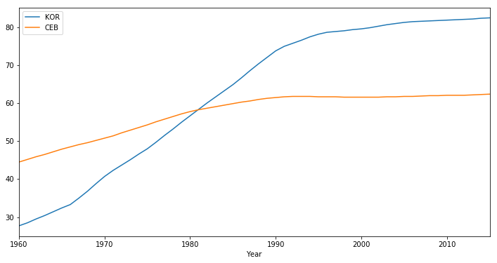
# example 3
year_s = pd.Series(list(df_k['Year']))
kor_s = pd.Series(list(df_k['UrbanPopRatio']))
ceb_s = pd.Series(list(df_c['UrbanPopRatio']))

df_new = pd.DataFrame()
df_new['Year'] = year_s
df_new['KOR'] = kor_s
df_new['CEB'] = ceb_s

df_new.head()
| Year | KOR | CEB | |
|---|---|---|---|
| 0 | 1960 | 27.7 | 44.5 |
| 1 | 1961 | 28.5 | 45.2 |
| 2 | 1962 | 29.5 | 45.9 |
| 3 | 1963 | 30.4 | 46.5 |
| 4 | 1964 | 31.4 | 47.2 |
df_new.plot(x='Year', y=['KOR','CEB'])
<matplotlib.axes._subplots.AxesSubplot at 0x111583eb8>
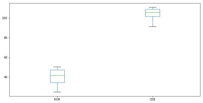
boxplot
kor_s = pd.Series(list(df_k['TotalPop']))
ceb_s = pd.Series(list(df_c['TotalPop']))

df_new = pd.DataFrame()
df_new['KOR'] = kor_s
df_new['CEB'] = ceb_s

df_new.head()
| KOR | CEB | |
|---|---|---|
| 0 | 25.0 | 91.4 |
| 1 | 25.8 | 92.2 |
| 2 | 26.5 | 93.0 |
| 3 | 27.3 | 93.8 |
| 4 | 28.0 | 94.7 |
cols = ['KOR', 'CEB']
df_new[cols].plot(kind='box')
<matplotlib.axes._subplots.AxesSubplot at 0x111624198>
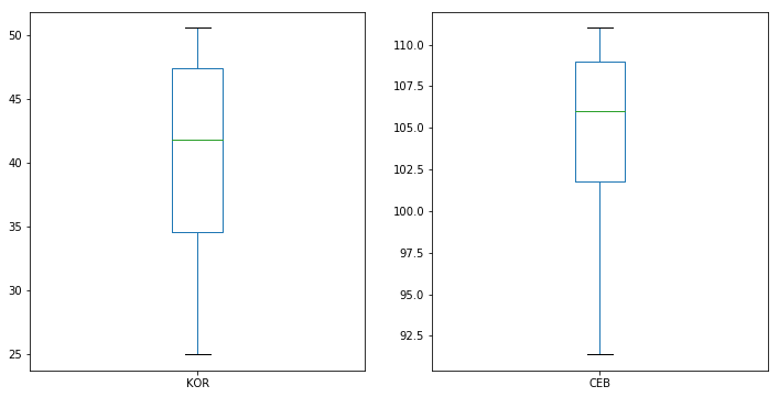
cols = ['KOR', 'CEB']
df_new[cols].plot(kind='box', subplots=True)   # Generate the box plots
KOR       Axes(0.125,0.125;0.352273x0.755)
CEB    Axes(0.547727,0.125;0.352273x0.755)
dtype: object
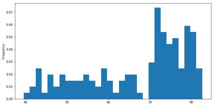
histogram
- histogram, scatter plot – pandas04 참조
df = pd.read_csv('data/worldreport.csv', index_col=0)
df.head()
| gdp_cap | life_exp | popul | |
|---|---|---|---|
| 0 | 974.58 | 43.82 | 31.88 |
| 1 | 5937.02 | 76.42 | 3.60 |
| 2 | 6223.36 | 72.30 | 33.33 |
| 3 | 4797.23 | 42.73 | 12.42 |
| 4 | 12779.37 | 75.31 | 40.30 |
df.describe()
| gdp_cap | life_exp | popul | |
|---|---|---|---|
| count | 142.000000 | 142.000000 | 142.000000 |
| mean | 11680.066831 | 67.002908 | 44.016514 |
| std | 12859.936734 | 12.073475 | 147.621369 |
| min | 277.550000 | 39.610000 | 0.190000 |
| 25% | 1624.837500 | 57.152500 | 4.505000 |
| 50% | 6124.365000 | 71.934000 | 10.515000 |
| 75% | 18008.830000 | 76.411000 | 31.202500 |
| max | 49357.190000 | 82.600000 | 1318.680000 |
df['life_exp'].plot(kind='hist', normed=True, bins=30)
<matplotlib.axes._subplots.AxesSubplot at 0x111ab67b8>
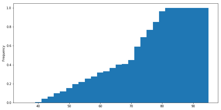
# 누적 히스토그램
df['life_exp'].plot(kind='hist', normed=True, cumulative=True, bins=30, range=(35,95))
<matplotlib.axes._subplots.AxesSubplot at 0x111ca2400>
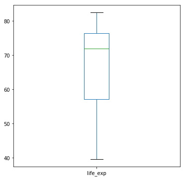
boxplot
df['life_exp'].plot(kind='box', figsize=(6,6))
<matplotlib.axes._subplots.AxesSubplot at 0x111e37fd0>
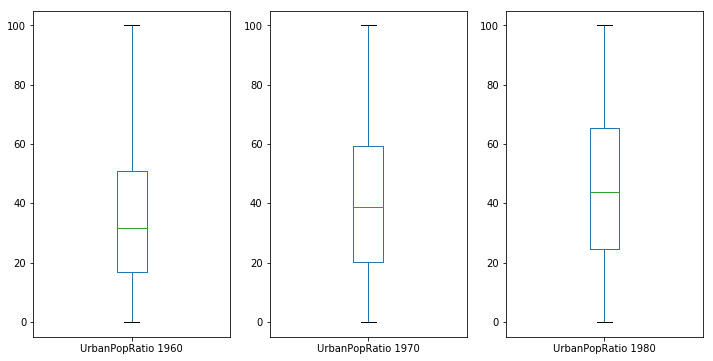
# subplot 분리
fig, axes = plt.subplots(nrows=1, ncols=3)
df_pop.loc[df_pop['Year'] == 1960].plot(ax=axes[0], y='UrbanPopRatio', kind='box', label='UrbanPopRatio 1960')
df_pop.loc[df_pop['Year'] == 1970].plot(ax=axes[1], y='UrbanPopRatio', kind='box', label='UrbanPopRatio 1970')
df_pop.loc[df_pop['Year'] == 1980].plot(ax=axes[2], y='UrbanPopRatio', kind='box', label='UrbanPopRatio 1980')
<matplotlib.axes._subplots.AxesSubplot at 0x1123d0c50>
Time Series
pandas03 참조
# df = pd.read_csv(filename, index_col='Date', parse_dates=True)
df_time = pd.read_csv('data/Product_airtime.csv')
df_time.head()
| PRODUCT_ID | AIR_DATE | PRODUCT_AIRTIME_MINS | PRODUCT_START_TMS | PRODUCT_STOP_TMS | |
|---|---|---|---|---|---|
| 0 | 2186 | 2012-10-16 0:00 | 0.38 | 2012-10-16 0:43 | 2012-10-16 0:44 |
| 1 | 2186 | 2012-10-16 0:00 | 5.08 | 2012-10-16 0:48 | 2012-10-16 0:53 |
| 2 | 2478 | 2012-10-16 0:00 | 0.50 | 2012-10-16 0:25 | 2012-10-16 0:26 |
| 3 | 2478 | 2012-10-16 0:00 | 12.53 | 2012-10-16 0:31 | 2012-10-16 0:43 |
| 4 | 6283 | 2012-10-16 0:00 | 0.43 | 2012-10-16 0:47 | 2012-10-16 0:48 |
date_list = df_time['PRODUCT_START_TMS']
date_list[0:10]
0    2012-10-16 0:43
1    2012-10-16 0:48
2    2012-10-16 0:25
3    2012-10-16 0:31
4    2012-10-16 0:47
5    2012-10-16 0:53
6    2012-10-16 0:00
7    2012-10-16 0:53
8    2012-10-16 0:59
9    2012-10-16 0:19
Name: PRODUCT_START_TMS, dtype: object
# Convert date_list into a datetime object
time_format = '%Y-%m-%d %H:%M'
my_datetimes = pd.to_datetime(date_list, format=time_format)
my_datetimes[0:10]
0   2012-10-16 00:43:00
1   2012-10-16 00:48:00
2   2012-10-16 00:25:00
3   2012-10-16 00:31:00
4   2012-10-16 00:47:00
5   2012-10-16 00:53:00
6   2012-10-16 00:00:00
7   2012-10-16 00:53:00
8   2012-10-16 00:59:00
9   2012-10-16 00:19:00
Name: PRODUCT_START_TMS, dtype: datetime64[ns]
df_time = pd.read_csv('data/Product_airtime.csv', index_col='PRODUCT_START_TMS', parse_dates=True)
df_time.head()
| PRODUCT_ID | AIR_DATE | PRODUCT_AIRTIME_MINS | PRODUCT_STOP_TMS | |
|---|---|---|---|---|
| PRODUCT_START_TMS | ||||
| 2012-10-16 00:43:00 | 2186 | 2012-10-16 0:00 | 0.38 | 2012-10-16 0:44 |
| 2012-10-16 00:48:00 | 2186 | 2012-10-16 0:00 | 5.08 | 2012-10-16 0:53 |
| 2012-10-16 00:25:00 | 2478 | 2012-10-16 0:00 | 0.50 | 2012-10-16 0:26 |
| 2012-10-16 00:31:00 | 2478 | 2012-10-16 0:00 | 12.53 | 2012-10-16 0:43 |
| 2012-10-16 00:47:00 | 6283 | 2012-10-16 0:00 | 0.43 | 2012-10-16 0:48 |
TimeSeries 생성
dateRange = pd.date_range('2017/03/01', periods=20, freq='D')
ts = pd.Series(range(len(dateRange)), index=dateRange)
ts[0:10]
2017-03-01    0
2017-03-02    1
2017-03-03    2
2017-03-04    3
2017-03-05    4
2017-03-06    5
2017-03-07    6
2017-03-08    7
2017-03-09    8
2017-03-10    9
Freq: D, dtype: int64
ts1 = ts.loc['2017-03-09']
ts1
8
ts2 = ts.loc['2017-03-05':'2017-03-10']
ts2
2017-03-05    4
2017-03-06    5
2017-03-07    6
2017-03-08    7
2017-03-09    8
2017-03-10    9
Freq: D, dtype: int64
sum12 = ts1 + ts2
sum12
2017-03-05    12
2017-03-06    13
2017-03-07    14
2017-03-08    15
2017-03-09    16
2017-03-10    17
Freq: D, dtype: int64
ts3 = ts2.reindex(ts.index)
ts3
2017-03-01    NaN
2017-03-02    NaN
2017-03-03    NaN
2017-03-04    NaN
2017-03-05    4.0
2017-03-06    5.0
2017-03-07    6.0
2017-03-08    7.0
2017-03-09    8.0
2017-03-10    9.0
2017-03-11    NaN
2017-03-12    NaN
2017-03-13    NaN
2017-03-14    NaN
2017-03-15    NaN
2017-03-16    NaN
2017-03-17    NaN
2017-03-18    NaN
2017-03-19    NaN
2017-03-20    NaN
Freq: D, dtype: float64
ts4 = ts2.reindex(ts.index, method='ffill')
ts4
2017-03-01    NaN
2017-03-02    NaN
2017-03-03    NaN
2017-03-04    NaN
2017-03-05    4.0
2017-03-06    5.0
2017-03-07    6.0
2017-03-08    7.0
2017-03-09    8.0
2017-03-10    9.0
2017-03-11    9.0
2017-03-12    9.0
2017-03-13    9.0
2017-03-14    9.0
2017-03-15    9.0
2017-03-16    9.0
2017-03-17    9.0
2017-03-18    9.0
2017-03-19    9.0
2017-03-20    9.0
Freq: D, dtype: float64
sum23 = ts2 + ts3
sum23
2017-03-01     NaN
2017-03-02     NaN
2017-03-03     NaN
2017-03-04     NaN
2017-03-05     8.0
2017-03-06    10.0
2017-03-07    12.0
2017-03-08    14.0
2017-03-09    16.0
2017-03-10    18.0
2017-03-11     NaN
2017-03-12     NaN
2017-03-13     NaN
2017-03-14     NaN
2017-03-15     NaN
2017-03-16     NaN
2017-03-17     NaN
2017-03-18     NaN
2017-03-19     NaN
2017-03-20     NaN
Freq: D, dtype: float64
Time Series Resample
df_time = pd.read_csv('data/Product_airtime.csv', index_col='PRODUCT_START_TMS', parse_dates=True)
df_time.head()
| PRODUCT_ID | AIR_DATE | PRODUCT_AIRTIME_MINS | PRODUCT_STOP_TMS | |
|---|---|---|---|---|
| PRODUCT_START_TMS | ||||
| 2012-10-16 00:43:00 | 2186 | 2012-10-16 0:00 | 0.38 | 2012-10-16 0:44 |
| 2012-10-16 00:48:00 | 2186 | 2012-10-16 0:00 | 5.08 | 2012-10-16 0:53 |
| 2012-10-16 00:25:00 | 2478 | 2012-10-16 0:00 | 0.50 | 2012-10-16 0:26 |
| 2012-10-16 00:31:00 | 2478 | 2012-10-16 0:00 | 12.53 | 2012-10-16 0:43 |
| 2012-10-16 00:47:00 | 6283 | 2012-10-16 0:00 | 0.43 | 2012-10-16 0:48 |
october = df_time['PRODUCT_AIRTIME_MINS']['2012-10']

# Downsample to obtain only the daily highest temperatures in August: august_highs
october_highs = october.resample('D').max()
print(october_highs)
PRODUCT_START_TMS
2012-10-01    17.05
2012-10-02    19.10
2012-10-03    21.63
2012-10-04    40.77
2012-10-05    12.23
2012-10-06    36.63
2012-10-07    56.57
2012-10-08    13.18
2012-10-09    25.47
2012-10-10    45.93
2012-10-11    29.10
2012-10-12    18.92
2012-10-13    18.27
2012-10-14    40.62
2012-10-15    14.78
2012-10-16    17.80
2012-10-17    31.70
2012-10-18    23.42
2012-10-19    22.32
2012-10-20    21.20
2012-10-21    36.72
2012-10-22    16.38
2012-10-23    22.35
2012-10-24    25.68
2012-10-25    21.08
2012-10-26    43.05
2012-10-27    35.77
2012-10-28    44.75
2012-10-29    17.37
2012-10-30    21.82
2012-10-31    30.13
Freq: D, Name: PRODUCT_AIRTIME_MINS, dtype: float64
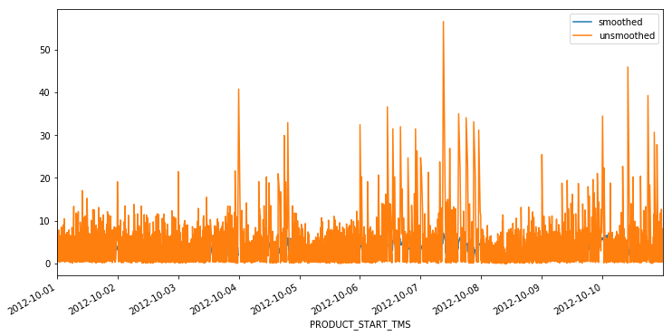
# Rolling means (or moving averages)
unsmoothed = df_time['PRODUCT_AIRTIME_MINS']['2012-10-01':'2012-10-10']

# Apply a rolling mean with a 24 hour window: smoothed
smoothed = unsmoothed.rolling(window=24).mean()

# Create a new DataFrame with columns smoothed and unsmoothed: august
august = pd.DataFrame({'smoothed':smoothed, 'unsmoothed':unsmoothed})

# Plot both smoothed and unsmoothed data using august.plot().
august.plot()
plt.show()
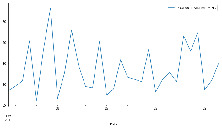
# Plotting time series, datetime indexing
october_highs.plot()
plt.legend()
plt.xlabel('Date')
<matplotlib.text.Text at 0x111e7f240>
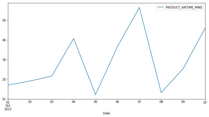
october_highs['2012-10-01':'2012-10-10'].plot()
plt.legend()
plt.xlabel('Date')
<matplotlib.text.Text at 0x10e0029e8>