Python Basics 1
Dictionary, Data Grouping, Loop
Dictionary
europe = {'spain':'madrid', 'france':'paris', 'germany':'berlin', 'norway':'oslo', 'australia':'vienna'}

print(europe.keys())
print(europe['norway'])
dict_keys(['france', 'australia', 'norway', 'spain', 'germany'])
oslo
europe['italy'] = 'rome'    # add or update
europe['poland'] = 'warsaw'
del(europe['australia'])    # Remove

print(europe)               # 순서는 고정 안됨
{'france': 'paris', 'spain': 'madrid', 'poland': 'warsaw', 'italy': 'rome', 'norway': 'oslo', 'germany': 'berlin'}
print('italy' in europe)
True
# Dictionary of dictionaries
europe = {'spain': {'capital':'madrid', 'population':46.77},
          'france': {'capital':'paris', 'population':66.03},
          'germany': {'capital':'berlin', 'population':80.62},
          'norway': {'capital':'oslo', 'population':5.084}}

print(europe['france']['capital'])
paris
# Create sub-dictionary data
data = {'capital':'rome', 'population':59.83}
europe['italy'] = data

print(europe)
{'france': {'population': 66.03, 'capital': 'paris'}, 'norway': {'population': 5.084, 'capital': 'oslo'}, 'italy': {'population': 59.83, 'capital': 'rome'}, 'spain': {'population': 46.77, 'capital': 'madrid'}, 'germany': {'population': 80.62, 'capital': 'berlin'}}
Pandas
import pandas as pd
import numpy as np
names = ['United States', 'Australia', 'Japan', 'India', 'Russia', 'Morocco', 'Egypt']
dr =  [True, False, False, False, True, True, True]
cpc = [809, 731, 588, 18, 200, 70, 45]

my_dict = {
    'country':names,
    'drives_right':dr,
    'cars_per_cap':cpc
}
# Build a DataFrame
cars = pd.DataFrame(my_dict)
cars.index = ['US', 'AUS', 'JAP', 'IN', 'RU', 'MOR', 'EG']
cars
| cars_per_cap | country | drives_right | |
|---|---|---|---|
| US | 809 | United States | True |
| AUS | 731 | Australia | False |
| JAP | 588 | Japan | False |
| IN | 18 | India | False |
| RU | 200 | Russia | True |
| MOR | 70 | Morocco | True |
| EG | 45 | Egypt | True |
cars = pd.read_csv('data/cars.csv', index_col = 0)
cars
| country | cars_per_cap | drives_right | |
|---|---|---|---|
| US | United States | 809 | True |
| AUS | Australia | 731 | False |
| JAP | Japan | 588 | False |
| IN | India | 18 | False |
| RU | Russia | 200 | True |
| MOR | Morocco | 70 | True |
| EG | Egypt | 45 | True |
print("\n{}".format(cars[1:4]))
print("\n{}".format(cars["country"]))      # output as Pandas Series
print("\n{}".format(cars[["country"]]))    # output as Pandas DataFrame
print("\n{}".format(cars[["country", "drives_right"]]))
       country  cars_per_cap drives_right
AUS  Australia           731        False
JAP      Japan           588        False
IN       India            18        False

US     United States
AUS        Australia
JAP            Japan
IN             India
RU            Russia
MOR          Morocco
EG             Egypt
Name: country, dtype: object

           country
US   United States
AUS      Australia
JAP          Japan
IN           India
RU          Russia
MOR        Morocco
EG           Egypt

           country drives_right
US   United States         True
AUS      Australia        False
JAP          Japan        False
IN           India        False
RU          Russia         True
MOR        Morocco         True
EG           Egypt         True
# loc & iloc
print(cars.loc[['RU', 'AUS']])
print(cars.iloc[[4, 1]])
       country  cars_per_cap drives_right
RU      Russia           200         True
AUS  Australia           731        False
       country  cars_per_cap drives_right
RU      Russia           200         True
AUS  Australia           731        False
print(cars.loc['MOR', 'drives_right'])
print(cars.loc[['RU','MOR'], ['country', 'drives_right']])  # sub-DataFrame
True
     country drives_right
RU    Russia         True
MOR  Morocco         True
print(cars.loc[:, 'drives_right'])      # Series
print(cars.loc[:, ['drives_right']])    # DataFrame
print(cars.loc[:, ['cars_per_cap', 'drives_right']])
US      True
AUS    False
JAP    False
IN     False
RU      True
MOR     True
EG      True
Name: drives_right, dtype: bool
    drives_right
US          True
AUS        False
JAP        False
IN         False
RU          True
MOR         True
EG          True
     cars_per_cap drives_right
US            809         True
AUS           731        False
JAP           588        False
IN             18        False
RU            200         True
MOR            70         True
EG             45         True
# Filtering pandas dataframe
cars[cars['drives_right'] == True]
| country | cars_per_cap | drives_right | |
|---|---|---|---|
| US | United States | 809 | True |
| RU | Russia | 200 | True |
| MOR | Morocco | 70 | True |
| EG | Egypt | 45 | True |
many_cars = cars["cars_per_cap"] > 500
cars[many_cars]
| country | cars_per_cap | drives_right | |
|---|---|---|---|
| US | United States | 809 | True |
| AUS | Australia | 731 | False |
| JAP | Japan | 588 | False |
Pandas Grouping
car = pd.read_csv('data/automobile.csv')
print(car.shape)
car.head()
(159, 26)
| symboling | normalized_losses | maker | fuel | aspiration | doors | body | wheels | engine_location | wheel_base | ... | engine_size | fuel_system | bore | stroke | compression_ratio | horsepower | peak_rpm | city_mpg | highway_mpg | price | |
|---|---|---|---|---|---|---|---|---|---|---|---|---|---|---|---|---|---|---|---|---|---|
| 0 | 2 | 164 | audi | gas | std | four | sedan | fwd | front | 99.8 | ... | 109 | mpfi | 3.19 | 3.4 | 10.0 | 102 | 5500 | 24 | 30 | 13950 |
| 1 | 2 | 164 | audi | gas | std | four | sedan | 4wd | front | 99.4 | ... | 136 | mpfi | 3.19 | 3.4 | 8.0 | 115 | 5500 | 18 | 22 | 17450 |
| 2 | 1 | 158 | audi | gas | std | four | sedan | fwd | front | 105.8 | ... | 136 | mpfi | 3.19 | 3.4 | 8.5 | 110 | 5500 | 19 | 25 | 17710 |
| 3 | 1 | 158 | audi | gas | turbo | four | sedan | fwd | front | 105.8 | ... | 131 | mpfi | 3.13 | 3.4 | 8.3 | 140 | 5500 | 17 | 20 | 23875 |
| 4 | 2 | 192 | bmw | gas | std | two | sedan | rwd | front | 101.2 | ... | 108 | mpfi | 3.50 | 2.8 | 8.8 | 101 | 5800 | 23 | 29 | 16430 |
5 rows × 26 columns
car.loc[car.wheels == '4wd']
| symboling | normalized_losses | maker | fuel | aspiration | doors | body | wheels | engine_location | wheel_base | ... | engine_size | fuel_system | bore | stroke | compression_ratio | horsepower | peak_rpm | city_mpg | highway_mpg | price | |
|---|---|---|---|---|---|---|---|---|---|---|---|---|---|---|---|---|---|---|---|---|---|
| 1 | 2 | 164 | audi | gas | std | four | sedan | 4wd | front | 99.4 | ... | 136 | mpfi | 3.19 | 3.40 | 8.0 | 115 | 5500 | 18 | 22 | 17450 |
| 99 | 2 | 83 | subaru | gas | std | two | hatchback | 4wd | front | 93.3 | ... | 108 | 2bbl | 3.62 | 2.64 | 8.7 | 73 | 4400 | 26 | 31 | 7603 |
| 103 | 0 | 102 | subaru | gas | std | four | sedan | 4wd | front | 97.0 | ... | 108 | 2bbl | 3.62 | 2.64 | 9.0 | 82 | 4800 | 24 | 25 | 9233 |
| 104 | 0 | 102 | subaru | gas | turbo | four | sedan | 4wd | front | 97.0 | ... | 108 | mpfi | 3.62 | 2.64 | 7.7 | 111 | 4800 | 24 | 29 | 11259 |
| 107 | 0 | 85 | subaru | gas | std | four | wagon | 4wd | front | 96.9 | ... | 108 | 2bbl | 3.62 | 2.64 | 9.0 | 82 | 4800 | 23 | 29 | 8013 |
| 108 | 0 | 85 | subaru | gas | turbo | four | wagon | 4wd | front | 96.9 | ... | 108 | mpfi | 3.62 | 2.64 | 7.7 | 111 | 4800 | 23 | 23 | 11694 |
| 113 | 0 | 81 | toyota | gas | std | four | wagon | 4wd | front | 95.7 | ... | 92 | 2bbl | 3.05 | 3.03 | 9.0 | 62 | 4800 | 27 | 32 | 7898 |
| 114 | 0 | 91 | toyota | gas | std | four | wagon | 4wd | front | 95.7 | ... | 92 | 2bbl | 3.05 | 3.03 | 9.0 | 62 | 4800 | 27 | 32 | 8778 |
8 rows × 26 columns
# symboling : 차량 안전등급 지수
car.loc[car.wheels == '4wd', 'symboling']
1      2
99     2
103    0
104    0
107    0
108    0
113    0
114    0
Name: symboling, dtype: int64
a1 = car.loc[car.wheels == '4wd', 'symboling'].mean()
a2 = car.loc[car.wheels == 'fwd', 'symboling'].mean()
print(a1);print(a2)
0.5
0.8952380952380953
grouped = car.groupby('wheels')
grouped.get_group('4wd')
| symboling | normalized_losses | maker | fuel | aspiration | doors | body | wheels | engine_location | wheel_base | ... | engine_size | fuel_system | bore | stroke | compression_ratio | horsepower | peak_rpm | city_mpg | highway_mpg | price | |
|---|---|---|---|---|---|---|---|---|---|---|---|---|---|---|---|---|---|---|---|---|---|
| 1 | 2 | 164 | audi | gas | std | four | sedan | 4wd | front | 99.4 | ... | 136 | mpfi | 3.19 | 3.40 | 8.0 | 115 | 5500 | 18 | 22 | 17450 |
| 99 | 2 | 83 | subaru | gas | std | two | hatchback | 4wd | front | 93.3 | ... | 108 | 2bbl | 3.62 | 2.64 | 8.7 | 73 | 4400 | 26 | 31 | 7603 |
| 103 | 0 | 102 | subaru | gas | std | four | sedan | 4wd | front | 97.0 | ... | 108 | 2bbl | 3.62 | 2.64 | 9.0 | 82 | 4800 | 24 | 25 | 9233 |
| 104 | 0 | 102 | subaru | gas | turbo | four | sedan | 4wd | front | 97.0 | ... | 108 | mpfi | 3.62 | 2.64 | 7.7 | 111 | 4800 | 24 | 29 | 11259 |
| 107 | 0 | 85 | subaru | gas | std | four | wagon | 4wd | front | 96.9 | ... | 108 | 2bbl | 3.62 | 2.64 | 9.0 | 82 | 4800 | 23 | 29 | 8013 |
| 108 | 0 | 85 | subaru | gas | turbo | four | wagon | 4wd | front | 96.9 | ... | 108 | mpfi | 3.62 | 2.64 | 7.7 | 111 | 4800 | 23 | 23 | 11694 |
| 113 | 0 | 81 | toyota | gas | std | four | wagon | 4wd | front | 95.7 | ... | 92 | 2bbl | 3.05 | 3.03 | 9.0 | 62 | 4800 | 27 | 32 | 7898 |
| 114 | 0 | 91 | toyota | gas | std | four | wagon | 4wd | front | 95.7 | ... | 92 | 2bbl | 3.05 | 3.03 | 9.0 | 62 | 4800 | 27 | 32 | 8778 |
8 rows × 26 columns
grouped['symboling'].mean()
wheels
4wd    0.500000
fwd    0.895238
rwd    0.413043
Name: symboling, dtype: float64
print(grouped['symboling'].agg([np.mean, np.sum]))
print(grouped['symboling'].agg({'평균': np.mean, '합계': np.sum}))
            mean  sum
wheels
4wd     0.500000    4
fwd     0.895238   94
rwd     0.413043   19
              평균  합계
wheels
4wd     0.500000   4
fwd     0.895238  94
rwd     0.413043  19
# Ordered Dictionary
from collections import OrderedDict
d = OrderedDict([('평균', np.mean), ('합계', np.sum)])
d
OrderedDict([('평균', <function numpy.core.fromnumeric.mean>),
             ('합계', <function numpy.core.fromnumeric.sum>)])
d['평균']
<function numpy.core.fromnumeric.mean>
grouped['symboling'].agg(OrderedDict([('평균', np.mean), ('합계', np.sum)]))
| 평균 | 합계 | |
|---|---|---|
| wheels | ||
| 4wd | 0.500000 | 4 |
| fwd | 0.895238 | 94 |
| rwd | 0.413043 | 19 |
Loop
distance = [11.25, 18.0, 20.0, 10.75, 9.50]
for d in distance :
    print(d)
11.25
18.0
20.0
10.75
9.5
enumerate
for index, a in enumerate(distance) :
    print("room " + str(index + 1) + " : " + str(a))
room 1 : 11.25
room 2 : 18.0
room 3 : 20.0
room 4 : 10.75
room 5 : 9.5
Loop over list
distance = [["London", 11.25],
            ["Rome", 18.0],
            ["Oslo", 20.0],
            ["Paris", 10.75],
            ["Madrid", 9.50]]
for city in distance:
    print("the " + city[0] + " : " + str(city[1]) + " km")
the London : 11.25 km
the Rome : 18.0 km
the Oslo : 20.0 km
the Paris : 10.75 km
the Madrid : 9.5 km
Loop over dictionary
europe = {'spain':'madrid', 'france':'paris', 'germany':'bonn', 'norway':'oslo', 'italy':'rome',
          'poland':'warsaw', 'australia':'vienna'}
for key, value in europe.items():
    print("the capital of " + key.upper() + " is " + value)
the capital of FRANCE is paris
the capital of AUSTRALIA is vienna
the capital of SPAIN is madrid
the capital of POLAND is warsaw
the capital of ITALY is rome
the capital of NORWAY is oslo
the capital of GERMANY is bonn
Loop over Numpy array
height = [74, 79, 72, 77, 73, 69, 67, 71, 76]
np_height = np.array(height)

for x in np_height :                # 1D array
    print(str(x) + " inches")
74 inches
79 inches
72 inches
77 inches
73 inches
69 inches
67 inches
71 inches
76 inches
people = [[74, 180], [74, 215], [72, 210], [72, 210], [73, 188], [69, 176]]
np_people = np.array(people)

for x in np_people :   # 2D array
    print(x)
[ 74 180]
[ 74 215]
[ 72 210]
[ 72 210]
[ 73 188]
[ 69 176]
for x in np.nditer(np_people) :   # 2D array
    print(x)
74
180
74
215
72
210
72
210
73
188
69
176
Loop over DataFrame
cars = pd.read_csv('data/cars.csv', index_col = 0)
for lab, row in cars.iterrows() :
    print(lab + " --- " + row['country'] + " : " + str(row['cars_per_cap']))
US --- United States : 809
AUS --- Australia : 731
JAP --- Japan : 588
IN --- India : 18
RU --- Russia : 200
MOR --- Morocco : 70
EG --- Egypt : 45
# adds COUNTRY column
for lab, row in cars.iterrows() :
    cars.loc[lab, 'COUNTRY'] = row['country'].upper()

cars
| country | cars_per_cap | drives_right | COUNTRY | |
|---|---|---|---|---|
| US | United States | 809 | True | UNITED STATES |
| AUS | Australia | 731 | False | AUSTRALIA |
| JAP | Japan | 588 | False | JAPAN |
| IN | India | 18 | False | INDIA |
| RU | Russia | 200 | True | RUSSIA |
| MOR | Morocco | 70 | True | MOROCCO |
| EG | Egypt | 45 | True | EGYPT |
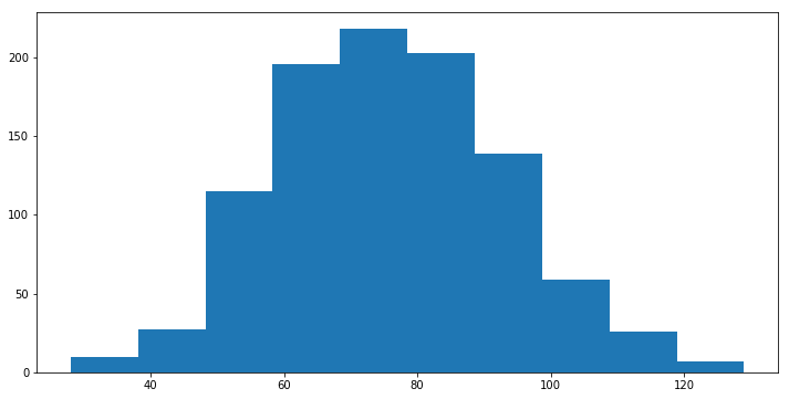
Case Study: Hacker Statistics. Normal Distribution
np.random.seed(9999)
print(np.random.rand())             # random float
print(np.random.randint(1, 7))      # random int (1~6 범위)
0.8233890742543671
2
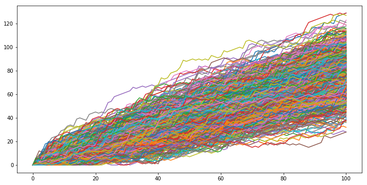
# Random Walk
all_walks = []
for i in range(1000) :
    random_walk = [0]

    for x in range(100) :
        # step에 마지막 숫자 설정
        step = random_walk[-1]

        # 주사위 던지기
        dice = np.random.randint(1,7)

        # 다음 step 결정.
        # 주사위 2 이하이면 -1. 3에서 5 사이이면 +1.
        if dice <= 2:
            step = max(0, step - 1)     # 음수값 되면 0 리턴
        elif dice <= 5:
            step += 1
        else:
            step += np.random.randint(1, 7)

        # append next_step to random_walk
        random_walk.append(step)

    # random_walk 결과를 전체 결과 array에 추가
    all_walks.append(random_walk)
np_all_walks = np.array(all_walks)
np_all_walks
array([[ 0,  6,  7, ..., 62, 61, 63],
       [ 0,  1,  2, ..., 67, 66, 65],
       [ 0,  1,  2, ..., 70, 71, 72],
       ...,
       [ 0,  0,  1, ..., 44, 43, 44],
       [ 0,  1,  2, ..., 51, 52, 53],
       [ 0,  0,  0, ..., 79, 84, 85]])
np_aw_t = np.transpose(np_all_walks)
np_aw_t
array([[ 0,  0,  0, ...,  0,  0,  0],
       [ 6,  1,  1, ...,  0,  1,  0],
       [ 7,  2,  2, ...,  1,  2,  0],
       ...,
       [62, 67, 70, ..., 44, 51, 79],
       [61, 66, 71, ..., 43, 52, 84],
       [63, 65, 72, ..., 44, 53, 85]])
%matplotlib inline
import matplotlib.pyplot as plt
# setting plot defatult size
%pylab inline
pylab.rcParams['figure.figsize'] = (12, 6)
Populating the interactive namespace from numpy and matplotlib
plt.plot(np_aw_t)
plt.show()
ends = np_aw_t[-1]
ends[0:50]
array([ 63,  65,  72,  51,  47,  47,  62,  42,  91,  71,  75,  82,  65,
        66,  80,  68,  64, 103,  80, 104,  81,  91,  75,  87,  75,  98,
        97, 118,  83,  81,  71,  41, 108,  66,  41,  84,  54,  76,  71,
        55,  65, 100,  69,  62,  81,  71,  57,  70, 112,  68])
plt.hist(ends)
plt.show()