이론 설명 링크
1. Random Forest
Randomization
- Bootstrap samples (Bagging)
- Random selection of K <= p split variables (Random input selection)

장단점
- 숲의 크기(나무의 수)가 커질수록 일반화오류가 특정값으로 수렴하게 되어 over-fitting을 피할 수 있음
- 전체 학습용 데이터에서 무작위로 복원추출된 데이터를 사용함으로써 잡음이나 outlier로부터 크게 영향을 받지 않음
- 분석가가 입력변수 선정으로부터 자유로울 수 있음
- Class의 빈도가 불균형일 경우 타기법에 비해 우수한 예측력을 보임
- 최종결과에 대한 해석이 어려움
library(randomForest)
library(caret)
library(ROCR)
# 홈쇼핑 반품 고객 예측

cb <- read.delim("data/Hshopping.txt", stringsAsFactors=FALSE)
cb$반품여부 <- factor(cb$반품여부)

set.seed(1)
inTrain <- createDataPartition(y=cb$반품여부, p=0.6, list=FALSE)
cb.train <- cb[inTrain,]
cb.test <- cb[-inTrain,]

# 모델링
# mtry : Number of variables randomly sampled as candidates at each split.
# ntree : Number of trees to grow.

set.seed(123)
rf_model <- randomForest(반품여부 ~ .-ID, data=cb.train, ntree=50, mtry=2)

rf_model     # OOB estimate : out-of-bag 샘플을 사용하여 검증
##
## Call:
##  randomForest(formula = 반품여부 ~ . - ID, data = cb.train, ntree = 50,      mtry = 2)
##                Type of random forest: classification
##                      Number of trees: 50
## No. of variables tried at each split: 2
##
##         OOB estimate of  error rate: 9.3%
## Confusion matrix:
##     0  1 class.error
## 0 193 14  0.06763285
## 1  14 80  0.14893617
plot(rf_model, main="random Forest model")
legend("topright", c("worst","overall","best"), fill = c("green", "black", "red"))

# 변수의 중요도
importance(rf_model)
##          MeanDecreaseGini
## 성별             7.648143
## 나이            65.864872
## 구매금액        17.421254
## 출연자          18.225289
varImpPlot(rf_model)

cb.test$rf_pred <- predict(rf_model, cb.test, type="response")
confusionMatrix(cb.test$rf_pred, cb.test$반품여부)
## Confusion Matrix and Statistics
##
##           Reference
## Prediction   0   1
##          0 125  11
##          1  12  51
##
##                Accuracy : 0.8844
##                  95% CI : (0.8316, 0.9253)
##     No Information Rate : 0.6884
##     P-Value [Acc > NIR] : 7.026e-11
##
##                   Kappa : 0.7318
##  Mcnemar's Test P-Value : 1
##
##             Sensitivity : 0.9124
##             Specificity : 0.8226
##          Pos Pred Value : 0.9191
##          Neg Pred Value : 0.8095
##              Prevalence : 0.6884
##          Detection Rate : 0.6281
##    Detection Prevalence : 0.6834
##       Balanced Accuracy : 0.8675
##
##        'Positive' Class : 0
##
cb.test$rf_pred_prob <- predict(rf_model, cb.test, type="prob")
rf_pred <- prediction(cb.test$rf_pred_prob[,2],cb.test$반품여부)

rf_model.perf1 <- performance(rf_pred, "tpr", "fpr")
plot(rf_model.perf1, colorize=TRUE); abline(a=0, b=1, lty=3)  # ROC-chart

rf_model.perf2 <- performance(rf_pred, "lift", "rpp")
plot(rf_model.perf2, colorize=TRUE); abline(v=0.4, lty=3)     # Lift chart

performance(rf_pred, "auc")@y.values[[1]]
## [1] 0.9574405
2. Support Vector Machine (SVM)
참고자료1
참고자료2
- 두 카테고리 중 어느 하나에 속한 데이터의 집합이 주어졌을 때, SVM 알고리즘은 주어진 데이터 집합을 바탕으로 새로운 데이터가 어느 카테고리에 속할지 판단하는 비확률적 이진 선형 분류모델을 만든다.
- 만들어진 분류모델은 데이터가 사상된 공간에서 경계로 표현되는데 SVM 알고리즘은 그 중 가장 큰 폭을 가진 경계를 찾는 알고리즘이다.
- SVM은 선형분류와 더불어 비선형 분류에서도 사용될 수 있다.
- 비선형분류를 하기 위해서 주어진 데이터를 고차원 특징 공간으로 사상하는 작업이 필요한데, 이를 효율적으로 하기 위해 '커널트릭'을 사용하기도 한다.
- Support Vector = 의사결정 경계에서 가장 가까운 데이터.

SVM의 특징
- 기존의 지도학습 모형과 같이 예측 부분에서 활용될 수 있으며 기계학습 부분에서 다른 모델에 비해 예측률이 높다고 알려져 있다.
- 넓은 형태의 데이터셋(많은 예측변수를 가지고 있는)에 적합하다.
- 모델을 생성할 때는 기본적인 설정사항을 이용해 비교적 빨리 모형을 생성할 수 있다.
- 실제 응용에 있어서 인공신경망보다 높은 성과를 내고 명백한 이론적 근거에 기반하므로 결과해석이 상대적으로 용이하다.
library(e1071)

# svm 주요 옵션
# cost : Complexity parameter (C).
# gamma : gamma parameter. 커질수록 가우시안 커브가 좁아진다. 즉, 튀어나온 봉우리들이 많아진다.
# probability : 확률적 예측 허용.

svm_model <- svm(반품여부~성별+나이+구매금액+출연자, data=cb.train, cost=100, gamma=1, probability = TRUE)
summary(svm_model)
##
## Call:
## svm(formula = 반품여부 ~ 성별 + 나이 + 구매금액 + 출연자, data = cb.train,
##     cost = 100, gamma = 1, probability = TRUE)
##
##
## Parameters:
##    SVM-Type:  C-classification
##  SVM-Kernel:  radial
##        cost:  100
##       gamma:  1
##
## Number of Support Vectors:  77
##
##  ( 45 32 )
##
##
## Number of Classes:  2
##
## Levels:
##  0 1
plot(svm_model, data=cb.train, 구매금액~나이)
legend(50, 1.7, "x : support vector")

# + : support vector
plot(cmdscale(dist(cb.train[,2:5])), col=cb.train$반품여부, pch=c("o","+")[1:nrow(cb.train) %in% svm_model$index+1])

cb.test$svm_pred <- predict(svm_model, cb.test)
confusionMatrix(cb.test$rf_pred, cb.test$반품여부)
## Confusion Matrix and Statistics
##
##           Reference
## Prediction   0   1
##          0 125  11
##          1  12  51
##
##                Accuracy : 0.8844
##                  95% CI : (0.8316, 0.9253)
##     No Information Rate : 0.6884
##     P-Value [Acc > NIR] : 7.026e-11
##
##                   Kappa : 0.7318
##  Mcnemar's Test P-Value : 1
##
##             Sensitivity : 0.9124
##             Specificity : 0.8226
##          Pos Pred Value : 0.9191
##          Neg Pred Value : 0.8095
##              Prevalence : 0.6884
##          Detection Rate : 0.6281
##    Detection Prevalence : 0.6834
##       Balanced Accuracy : 0.8675
##
##        'Positive' Class : 0
##
postResample(cb.test$svm_pred, cb.test$반품여부)
##  Accuracy     Kappa
## 0.8844221 0.7293798
cb.test$svm_pred_prob <- attr(predict(svm_model, cb.test, probability = TRUE), "probabilities")[,2] # 1이 될 확률

svm_pred <- prediction(cb.test$svm_pred_prob, cb.test$반품여부)

svm_model.perf1 <- performance(svm_pred, "tpr", "fpr") # ROC-chart
plot(svm_model.perf1, colorize=TRUE); abline(a=0, b=1, lty=3)

svm_model.perf2 <- performance(svm_pred, "lift", "rpp")
plot(svm_model.perf2, colorize=TRUE); abline(v=0.4, lty=3)

performance(svm_pred, "auc")@y.values[[1]]
## [1] 0.9210031
# the best values to use for the parameters gamma and cost
set.seed(123)
tune.svm(반품여부~성별+나이+구매금액+출연자, data=cb.train, gamma=seq(.5, .9, by=.1), cost=seq(100,1000, by=100))
##
## Parameter tuning of 'svm':
##
## - sampling method: 10-fold cross validation
##
## - best parameters:
##  gamma cost
##    0.9  300
##
## - best performance: 0.1062366
3. K-fold Cross Validation
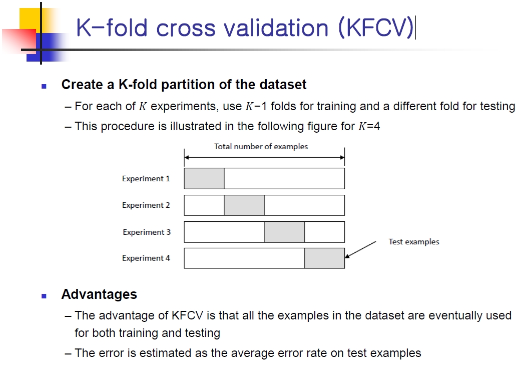
# Create a 5-fold partition using the caret package
set.seed(1)
flds <- createFolds(cb$반품여부, k=5, list=TRUE, returnTrain=FALSE)
str(flds)
## List of 5
##  $ Fold1: int [1:99] 5 7 12 14 18 19 21 25 30 32 ...
##  $ Fold2: int [1:101] 11 33 39 41 45 80 85 86 90 94 ...
##  $ Fold3: int [1:100] 10 15 16 22 24 31 34 35 36 48 ...
##  $ Fold4: int [1:100] 2 3 4 8 9 13 20 23 26 29 ...
##  $ Fold5: int [1:100] 1 6 17 27 28 43 46 47 53 54 ...
# Perform 5 experiments
experiment <- function(train, test, m) {
  rf <- randomForest(반품여부 ~ .-ID, data=train, ntree=50)
  rf_pred <- predict(rf, test, type="response")
  m$acc = c(m$acc, confusionMatrix(rf_pred, test$반품여부)$overall[1])   # 정확도
  rf_pred_prob <- predict(rf, test, type="prob")
  rf_pred <- prediction(rf_pred_prob[,2], cb.test$반품여부)    # 예측
  m$auc = c(m$auc, performance(rf_pred, "auc")@y.values[[1]])  # AUC
  return(m)
}

measure = list()
for(i in 1:5){
  inTest <- flds[[i]]
  cb.test <- cb[inTest, ]
  cb.train <- cb[-inTest, ]
  measure = experiment(cb.train, cb.test, measure)
}

measure
## $acc
##  Accuracy  Accuracy  Accuracy  Accuracy  Accuracy
## 0.8888889 0.8712871 0.9200000 0.9100000 0.9000000
##
## $auc
## [1] 0.9656072 0.9585598 0.9630669 0.9614306 0.9794296
mean(measure$acc); sd(measure$acc)
## [1] 0.8980352
## [1] 0.0188983
mean(measure$auc); sd(measure$auc)
## [1] 0.9656188
## [1] 0.008133616