Data Mining - Neural Network
# 홈쇼핑에서 반품 고객의 특성을 파악하고자 인공신경망 분석 활용
인공신경망 이론 (링크)
1. Neural Network Analysis using "nnet" package
library(nnet)
library(caret)
library(ROCR)
cb <- read.delim("data/Hshopping.txt", stringsAsFactors=FALSE)
head(cb)
##   ID 성별 나이 구매금액 출연자 반품여부
## 1  1    1   33        2      2        0
## 2  2    2   21        3      2        1
## 3  3    1   45        1      1        0
## 4  4    1   50        2      1        0
## 5  5    1   21        3      1        1
## 6  6    1   22        3      1        1
summary(cb$반품여부)
##    Min. 1st Qu.  Median    Mean 3rd Qu.    Max.
##   0.000   0.000   0.000   0.312   1.000   1.000
cb$반품여부 <- factor(cb$반품여부)  # 명목형 값 예측일 경우 factor로 변환.
summary(cb$반품여부)
##   0   1
## 344 156
# 데이터 분할
set.seed(1)
inTrain <- createDataPartition(y=cb$반품여부, p=0.6, list=FALSE)
cb.train <- cb[inTrain,]
cb.test <- cb[-inTrain,]
# 모델링

# nnet의 주요 옵션들
# size : hidden node 수
# maxit : 반복횟수
# decay : overfitting을 피하기 위해 사용하는 weight decay parameter
# rang : Initial random weights on [-rang, rang]. default 0.5
set.seed(123)

nn_model1 <- nnet(반품여부 ~ 성별+나이+구매금액+출연자, data=cb.train, size=3, maxit=1000)
## # weights:  19
## initial  value 200.606812
## iter  10 value 86.410893
## iter  20 value 81.774551
## iter  30 value 76.044092
## iter  40 value 66.203022
## iter  50 value 63.924238
## iter  60 value 63.114128
## iter  70 value 62.903511
    .........
## iter 400 value 49.402414
## iter 410 value 49.402301
## iter 420 value 49.401785
## iter 430 value 49.401572
## iter 440 value 49.401474
## iter 450 value 49.401280
## iter 460 value 49.400976
## final  value 49.400929
## converged
nn_model2 <- nnet(반품여부 ~ 성별+나이+구매금액+출연자, data=cb.train, size=5, maxit=1000, decay = 0.0005, rang = 0.1)
## # weights:  31
## initial  value 197.970465
## iter  10 value 75.903511
## iter  20 value 64.938108
## iter  30 value 60.738498
## iter  40 value 57.431605
## iter  50 value 55.116059
## iter  60 value 52.363732
## iter  70 value 51.978971
    .........
## iter 400 value 41.291765
## iter 410 value 41.277988
## iter 420 value 41.253266
## iter 430 value 41.245844
## iter 440 value 41.244417
## iter 450 value 41.243771
## final  value 41.243740
## converged
summary(nn_model1)
## a 4-3-1 network with 19 weights
## options were - entropy fitting
##   b->h1  i1->h1  i2->h1  i3->h1  i4->h1
##   26.33 -101.85    3.32  -69.49   47.08
##   b->h2  i1->h2  i2->h2  i3->h2  i4->h2
## -243.83  100.35   -7.51   97.79   20.53
##   b->h3  i1->h3  i2->h3  i3->h3  i4->h3
##  -86.52  -17.34    5.66   18.53  -74.97
##    b->o   h1->o   h2->o   h3->o
##    0.57  -35.69   53.31   -2.57
summary(nn_model2)
## a 4-5-1 network with 31 weights
## options were - entropy fitting  decay=5e-04
##  b->h1 i1->h1 i2->h1 i3->h1 i4->h1
##  17.56 -11.75   1.73   2.07 -30.40
##  b->h2 i1->h2 i2->h2 i3->h2 i4->h2
##  38.28 -18.18   0.89 -14.03   3.08
##  b->h3 i1->h3 i2->h3 i3->h3 i4->h3
##  15.28 -30.77   0.63 -14.48  16.85
##  b->h4 i1->h4 i2->h4 i3->h4 i4->h4
##   6.20 -15.06   0.42  -9.73   7.21
##  b->h5 i1->h5 i2->h5 i3->h5 i4->h5
##   2.56  20.42  -1.17   6.20   4.74
##   b->o  h1->o  h2->o  h3->o  h4->o  h5->o
##   5.48  -3.03 -13.77  21.03 -28.93   9.62
library(devtools)

source_url('https://gist.githubusercontent.com/Peque/41a9e20d6687f2f3108d/raw/85e14f3a292e126f1454864427e3a189c2fe33f3/nnet_plot_update.r')
plot.nnet(nn_model1)

plot.nnet(nn_model2)

# 위 인공신경망 모델에서 각 변수의 중요도 확인
library(NeuralNetTools)

garson(nn_model1)

garson(nn_model2)

# 두 모델의 테스트 데이터셋에 대한 예측력/성능 비교
# nn_model1
confusionMatrix(predict(nn_model1, newdata=cb.test, type="class"), cb.test$반품여부)
## Confusion Matrix and Statistics
##
##           Reference
## Prediction   0   1
##          0 121  12
##          1  16  50
##
##                Accuracy : 0.8593
##                  95% CI : (0.8031, 0.9044)
##     No Information Rate : 0.6884
##     P-Value [Acc > NIR] : 1.999e-08
##
##                   Kappa : 0.6777
##  Mcnemar's Test P-Value : 0.5708
##
##             Sensitivity : 0.8832
##             Specificity : 0.8065
##          Pos Pred Value : 0.9098
##          Neg Pred Value : 0.7576
##              Prevalence : 0.6884
##          Detection Rate : 0.6080
##    Detection Prevalence : 0.6683
##       Balanced Accuracy : 0.8448
##
##        'Positive' Class : 0
##
# nn_model2
confusionMatrix(predict(nn_model2, newdata=cb.test, type="class"), cb.test$반품여부)
## Confusion Matrix and Statistics
##
##           Reference
## Prediction   0   1
##          0 126  11
##          1  11  51
##
##                Accuracy : 0.8894
##                  95% CI : (0.8374, 0.9294)
##     No Information Rate : 0.6884
##     P-Value [Acc > NIR] : 1.98e-11
##
##                   Kappa : 0.7423
##  Mcnemar's Test P-Value : 1
##
##             Sensitivity : 0.9197
##             Specificity : 0.8226
##          Pos Pred Value : 0.9197
##          Neg Pred Value : 0.8226
##              Prevalence : 0.6884
##          Detection Rate : 0.6332
##    Detection Prevalence : 0.6884
##       Balanced Accuracy : 0.8711
##
##        'Positive' Class : 0
##
# ROCR::prediction - ROCR 패키지에 있는 prediction 함수 사용.

# model1
nn_pred1 <- ROCR::prediction(predict(nn_model1, newdata=cb.test, type="raw"), cb.test$반품여부)
nn_model1.roc <- performance(nn_pred1, "tpr", "fpr")   # ROC-chart
plot(nn_model1.roc, colorize=TRUE)

nn_model1.lift <- performance(nn_pred1, "lift", "rpp")  # Lift chart
plot(nn_model1.lift, colorize=TRUE)

# model2
nn_pred2 <- ROCR::prediction(predict(nn_model2, newdata=cb.test, type="raw"), cb.test$반품여부)
nn_model2.roc <- performance(nn_pred2, "tpr", "fpr")   # ROC-chart
plot(nn_model2.roc, colorize=TRUE)

nn_model2.lift <- performance(nn_pred2, "lift", "rpp")  # Lift chart
plot(nn_model2.lift, colorize=TRUE)

2. Neural Network Analysis using "neuralnet" package
library(neuralnet)
cb <- read.delim("data/Hshopping.txt", stringsAsFactors=FALSE) # neuralnet 패키지는 목표변수가 numeric.
# 데이터 분할
set.seed(1)
inTrain <- createDataPartition(y=cb$반품여부, p=0.6, list=FALSE)
cb.train <- cb[inTrain,]
cb.test <- cb[-inTrain,]
# 모델링
set.seed(123)
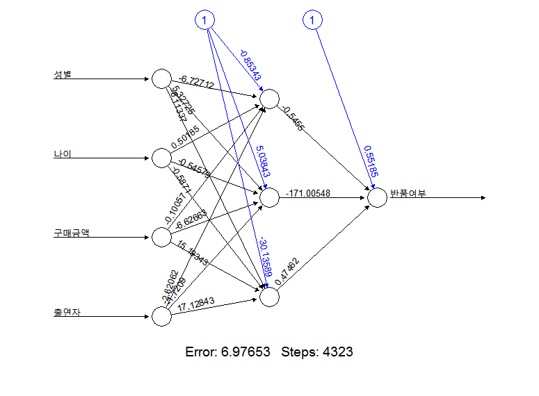
nnet_model1 <- neuralnet(반품여부 ~ 성별+나이+구매금액+출연자, data=cb.train, hidden=3, threshold=0.01)
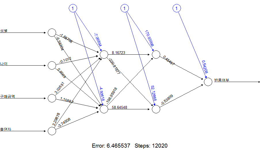
nnet_model2 <- neuralnet(반품여부 ~ 성별+나이+구매금액+출연자, data=cb.train, hidden=c(2,2), threshold=0.01)
# threshold : 에러의 감소분이 threshold 값보다 작으면 stop
# hidden : hidden node 수.
# hidden=c(2,2) : hidden layer 2개가 각각 hidden node 2개를 가짐
# linear.output: 활성함수('logistic' or 'tanh')가 출력 뉴런에 적용되지 않아야 하는 경우(즉, 회귀) TRUE로 설정(default)
# stepmax: 훈련 수행 최대 횟수
plot(nnet_model1)
plot(nnet_model2)
# 모델 내에서 각 변수의 영향도(일반화 가중치)
# 나이 : 분산이 0에 가까움. 결과에 미치는 영향이 미미하다.
par(mfrow=c(2,2))
gwplot(nnet_model1, selected.covariate = "성별", min=-3,max=6)
gwplot(nnet_model1, selected.covariate = "나이", min=-3,max=6)
gwplot(nnet_model1, selected.covariate = "구매금액", min=-3,max=6)
gwplot(nnet_model1, selected.covariate = "출연자", min=-3,max=6)

par(mfrow=c(1,1))


# 테스트 데이터에서 필요한 필드만 지정!!!
# nnet_model1
cb.test$nnet1_pred_prob <- compute(nnet_model1, covariate=cb.test[, c(2:5)])$net.result
cb.test$nnet1_pred <- ifelse(cb.test$nnet1_pred_prob > 0.5, 1, 0)
confusionMatrix(cb.test$nnet1_pred, cb.test$반품여부)
## Confusion Matrix and Statistics
##
##           Reference
## Prediction   0   1
##          0 128  13
##          1  13  46
##
##                Accuracy : 0.87
##                  95% CI : (0.8153477, 0.9132916)
##     No Information Rate : 0.705
##     P-Value [Acc > NIR] : 0.00000002942981
##
##                   Kappa : 0.6874624
##  Mcnemar's Test P-Value : 1
##
##             Sensitivity : 0.9078014
##             Specificity : 0.7796610
##          Pos Pred Value : 0.9078014
##          Neg Pred Value : 0.7796610
##              Prevalence : 0.7050000
##          Detection Rate : 0.6400000
##    Detection Prevalence : 0.7050000
##       Balanced Accuracy : 0.8437312
##
##        'Positive' Class : 0
##
# nnet_model2
cb.test$nnet2_pred_prob <- compute(nnet_model2, covariate=cb.test[, c(2:5)])$net.result
cb.test$nnet2_pred <- ifelse(cb.test$nnet2_pred_prob > 0.5, 1, 0)
confusionMatrix(cb.test$nnet2_pred, cb.test$반품여부)
## Confusion Matrix and Statistics
##
##           Reference
## Prediction   0   1
##          0 128  17
##          1  13  42
##
##                Accuracy : 0.85
##                  95% CI : (0.7928413, 0.8964505)
##     No Information Rate : 0.705
##     P-Value [Acc > NIR] : 0.000001340647
##
##                   Kappa : 0.6321275
##  Mcnemar's Test P-Value : 0.5838824
##
##             Sensitivity : 0.9078014
##             Specificity : 0.7118644
##          Pos Pred Value : 0.8827586
##          Neg Pred Value : 0.7636364
##              Prevalence : 0.7050000
##          Detection Rate : 0.6400000
##    Detection Prevalence : 0.7250000
##       Balanced Accuracy : 0.8098329
##
##        'Positive' Class : 0
##
# ROC & Lift chart
nnet1_pred <- ROCR::prediction(cb.test$nnet1_pred_prob, cb.test$반품여부)
nnet_model1.roc <- performance(nnet1_pred, "tpr", "fpr") # ROC-chart
plot(nnet_model1.roc, colorize=TRUE)

nnet_model1.lift <- performance(nnet1_pred, "lift", "rpp") # Lift chart
plot(nnet_model1.lift, colorize=TRUE)

nnet2_pred <- ROCR::prediction(cb.test$nnet2_pred_prob, cb.test$반품여부)
nnet_model2.roc <- performance(nnet2_pred, "tpr", "fpr") # ROC-chart
##### Input Normalization in Neural Networks

# 입력값 정규화
# 값을 0 ~ 1 사이의 값으로 변환
normalize <- function (x) {
    normalized = (x - min(x)) / (max(x) - min(x))
    return(normalized)
}

cb <- read.delim("data/Hshopping.txt", stringsAsFactors=FALSE)

# 나이와 구매금액을 정규화
cb$나이 <- normalize(cb$나이)
cb$구매금액 <- normalize(cb$구매금액)

head(cb)
##   ID 성별         나이 구매금액 출연자 반품여부
## 1  1    1 0.2666666667      0.5      2        0
## 2  2    2 0.1066666667      1.0      2        1
## 3  3    1 0.4266666667      0.0      1        0
## 4  4    1 0.4933333333      0.5      1        0
## 5  5    1 0.1066666667      1.0      1        1
## 6  6    1 0.1200000000      1.0      1        1
set.seed(1)
inTrain <- createDataPartition(y=cb$반품여부, p=0.6, list=FALSE)
cb.train <- cb[inTrain,]
cb.test <- cb[-inTrain,]

set.seed(123)
nnet_model3 <- neuralnet(반품여부 ~ 성별+나이+구매금액+출연자, data=cb.train, hidden=3, threshold=0.01)

par(mfrow=c(2,2))
gwplot(nnet_model3, selected.covariate = "성별", min=-3, max=6)
gwplot(nnet_model3, selected.covariate = "나이", min=-3, max=6)
gwplot(nnet_model3, selected.covariate = "구매금액", min=-3, max=6)
gwplot(nnet_model3, selected.covariate = "출연자", min=-3, max=6)

par(mfrow=c(1,1))

garson(nnet_model3)

cb.test$nnet3_pred_prob <- compute(nnet_model3, covariate=cb.test[, c(2:5)])$net.result
cb.test$nnet3_pred <- ifelse(cb.test$nnet3_pred_prob > 0.5, 1, 0)
confusionMatrix(cb.test$nnet3_pred, cb.test$반품여부)
## Confusion Matrix and Statistics
##
##           Reference
## Prediction   0   1
##          0 131  12
##          1  10  47
##
##                Accuracy : 0.89
##                  95% CI : (0.8382038, 0.9297668)
##     No Information Rate : 0.705
##     P-Value [Acc > NIR] : 0.0000000003254392
##
##                   Kappa : 0.7329125
##  Mcnemar's Test P-Value : 0.8311704
##
##             Sensitivity : 0.9290780
##             Specificity : 0.7966102
##          Pos Pred Value : 0.9160839
##          Neg Pred Value : 0.8245614
##              Prevalence : 0.7050000
##          Detection Rate : 0.6550000
##    Detection Prevalence : 0.7150000
##       Balanced Accuracy : 0.8628441
##
##        'Positive' Class : 0
##
# Model Comparison

nnet3_pred <- ROCR::prediction(cb.test$nnet3_pred_prob, cb.test$반품여부)
nnet_model3.roc <- performance(nnet3_pred, "tpr", "fpr") # ROC-chart

plot(nnet_model1.roc, col="red")
plot(nnet_model2.roc, col="green", add=T)
plot(nnet_model3.roc, col="blue", add=T)

legend(0.6,0.7,c("nnet_model1","nnet_model2","nnet_model3"),cex=0.9,col=c("red","green","blue"),lty=1)

performance(nnet1_pred, "auc")@y.values[[1]]
## [1] 0.8942781584
performance(nnet2_pred, "auc")@y.values[[1]]
## [1] 0.9343070081
performance(nnet3_pred, "auc")@y.values[[1]]
## [1] 0.9308210121
3. "Multinomial Classification" using neuralnet
# iris 데이터 다항 분류
data(iris)
summary(iris)
##   Sepal.Length       Sepal.Width        Petal.Length    Petal.Width
##  Min.   :4.300000   Min.   :2.000000   Min.   :1.000   Min.   :0.100000
##  1st Qu.:5.100000   1st Qu.:2.800000   1st Qu.:1.600   1st Qu.:0.300000
##  Median :5.800000   Median :3.000000   Median :4.350   Median :1.300000
##  Mean   :5.843333   Mean   :3.057333   Mean   :3.758   Mean   :1.199333
##  3rd Qu.:6.400000   3rd Qu.:3.300000   3rd Qu.:5.100   3rd Qu.:1.800000
##  Max.   :7.900000   Max.   :4.400000   Max.   :6.900   Max.   :2.500000
##        Species
##  setosa    :50
##  versicolor:50
##  virginica :50
# neuralnet은 식에서 '.'을 지원하지 않기 때문에 아래와 같이 식을 문자열로 생성.
formula <- as.formula(paste('Species ~ ', paste(names(iris)[-length(iris)], collapse='+')))
formula
## Species ~ Sepal.Length + Sepal.Width + Petal.Length + Petal.Width
# neuralnet does not support the '.' notation in the formula.
# multi_model <- neuralnet(formula, iris, hidden=3, linear.output=FALSE)

# fails !
# Species가 factor : neuralnet 패키지는 target으로 factor를 사용할 수 없다.
# Species를 3개의 binary 변수로 펼쳐야 한다.

formula <- as.formula(paste('setosa + versicolor + virginica ~ ', paste(names(iris)[-length(iris)], collapse='+')))
formula
## setosa + versicolor + virginica ~ Sepal.Length + Sepal.Width +
##     Petal.Length + Petal.Width
trainData <- cbind(iris[, 1:4], class.ind(iris$Species))
head(trainData)
##   Sepal.Length Sepal.Width Petal.Length Petal.Width setosa versicolor
## 1          5.1         3.5          1.4         0.2      1          0
## 2          4.9         3.0          1.4         0.2      1          0
## 3          4.7         3.2          1.3         0.2      1          0
## 4          4.6         3.1          1.5         0.2      1          0
## 5          5.0         3.6          1.4         0.2      1          0
## 6          5.4         3.9          1.7         0.4      1          0
##   virginica
## 1         0
## 2         0
## 3         0
## 4         0
## 5         0
## 6         0
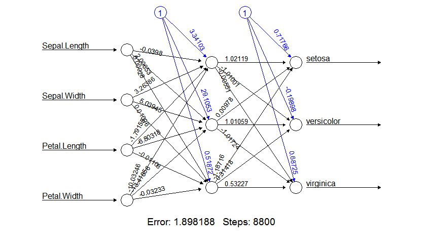
multi_model <- neuralnet(formula, trainData, hidden=3)
plot(multi_model)
species_prob = compute(multi_model, iris[, 1:4])$net.result
head(species_prob)
##              [,1]              [,2]              [,3]
## [1,] 0.9999999967 -0.00066075253881  0.00063389434950
## [2,] 0.9999999929  0.00101469292227 -0.00100920304022
## [3,] 0.9999999945  0.00030837464151 -0.00031652175015
## [4,] 0.9999999920  0.00141887532902 -0.00140558183794
## [5,] 0.9999999970 -0.00080825597291  0.00077854991315
## [6,] 0.9999999954 -0.00009871907406  0.00008271214732