Tensorflow Linear Regression
Tensorflow를 사용하여 간단하게 구현한 Linear Regression 예제
Computational Graph
import tensorflow as tf
a = tf.placeholder(tf.float32)
b = tf.placeholder(tf.float32)
c = a + b

sess = tf.Session()

print(sess.run(c, feed_dict={a: 3, b: 4.5}))
print(sess.run(c, feed_dict={a: [1, 3], b: [2, 4]}))
7.5
[ 3.  7.]
d = c * 3.
print(sess.run(d, feed_dict={a: 3, b:4.5}))
22.5
Linear Regression

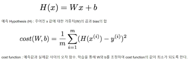
예측 Hypothesis (H) : 주어진 x 값에 대한 가중치(W)의 곱과 bias의 합
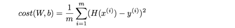
cost function : 예측값과 실제값 사이의 오차 함수. 학습을 통해 W와 b를 조정하여 cost function의 값이 최소가 되도록 한다.
Hypothesis
# data
x_train = [1, 2, 3]
y_train = [1, 2, 3]

# 변수. 임의의 값 설정.
W = tf.Variable(tf.random_normal([1]), name='weight')
b = tf.Variable(tf.random_normal([1]), name='bias')

hypothesis = x_train * W + b             # 실제값 : W = 1, b = 0
cost function
cost = tf.reduce_mean(tf.square(hypothesis - y_train)) # 평균
optimizer - minimize cost
optimizer = tf.train.GradientDescentOptimizer(learning_rate=0.01)
train = optimizer.minimize(cost)
run graph
sess = tf.Session()
sess.run(tf.global_variables_initializer())   # 변수 초기화 !!!
# Fit
for step in range(2001):
    sess.run(train)
    if step % 200 == 0:
        print(step, sess.run(cost), sess.run(W), sess.run(b))
0 6.28194 [ 1.63046098] [ 1.19202673]
200 0.0321736 [ 0.79167271] [ 0.47357684]
400 0.0122855 [ 0.87126642] [ 0.29264179]
600 0.00469118 [ 0.92045051] [ 0.18083476]
800 0.00179133 [ 0.95084321] [ 0.11174489]
1000 0.000684017 [ 0.96962404] [ 0.06905165]
1200 0.00026119 [ 0.9812296] [ 0.04266965]
1400 9.97355e-05 [ 0.988401] [ 0.02636725]
1600 3.80839e-05 [ 0.99283254] [ 0.01629329]
1800 1.45421e-05 [ 0.99557096] [ 0.01006831]
2000 5.55311e-06 [ 0.99726313] [ 0.00622157]
# W = 1, b = 0 에 가까워졌다.
Linear Regression - Placeholder & Feed
X = tf.placeholder(tf.float32, shape=[None])
Y = tf.placeholder(tf.float32, shape=[None])
W = tf.Variable(tf.random_normal([1]), name='weight')
b = tf.Variable(tf.random_normal([1]), name='bias')

hypothesis = X * W + b
cost = tf.reduce_mean(tf.square(hypothesis - Y))
optimizer = tf.train.GradientDescentOptimizer(learning_rate=0.01)
train = optimizer.minimize(cost)
sess = tf.Session()
sess.run(tf.global_variables_initializer())
# Fit
for step in range(2001):
    cost_val, W_val, b_val, _ = sess.run([cost, W, b, train], feed_dict={X: [1, 2, 3], Y: [1, 2, 3]})
    if step % 200 == 0:
        print(step, cost_val, W_val, b_val)
0 0.952772 [ 0.77082062] [-0.39007139]
200 0.00323303 [ 1.0658803] [-0.14976136]
400 0.00123454 [ 1.04071021] [-0.09254375]
600 0.000471408 [ 1.0251565] [-0.05718652]
800 0.000180003 [ 1.01554501] [-0.03533759]
1000 6.87344e-05 [ 1.00960588] [-0.02183652]
1200 2.62465e-05 [ 1.00593591] [-0.0134937]
1400 1.00227e-05 [ 1.00366807] [-0.00833846]
1600 3.82775e-06 [ 1.00226688] [-0.005153]
1800 1.46214e-06 [ 1.00140107] [-0.00318478]
2000 5.5866e-07 [ 1.00086606] [-0.00196877]
# Test model
print(sess.run(hypothesis, feed_dict={X: [1.5, 3.5]}))
[ 1.4993304 3.50106239]
# 새로운 training data로 Fit
for step in range(2001):
    cost_val, W_val, b_val, _ = sess.run([cost, W, b, train],
                                         feed_dict={X: [1,   2,   3,   4,   5],
                                                    Y: [2.1, 3.1, 4.1, 5.1, 6.1]})   # y = 1 * x + 1.1
    if step % 200 == 0:
        print(step, cost_val, W_val, b_val)
0 1.20862 [ 1.06679368] [ 0.02001864]
200 0.049216 [ 1.14354241] [ 0.58176589]
400 0.0126992 [ 1.07291496] [ 0.8367539]
600 0.00327678 [ 1.03703833] [ 0.9662798]
800 0.000845496 [ 1.01881397] [ 1.03207529]
1000 0.000218165 [ 1.00955689] [ 1.06549597]
1200 5.62957e-05 [ 1.00485468] [ 1.08247304]
1400 1.45265e-05 [ 1.00246608] [ 1.09109652]
1600 3.74845e-06 [ 1.00125265] [ 1.0954771]
1800 9.678e-07 [ 1.0006367] [ 1.09770191]
2000 2.50054e-07 [ 1.00032365] [ 1.09883177]
# Test model
print(sess.run(hypothesis, feed_dict={X: [1.5, 3.5]}))
[ 2.59931707 4.59996462]